Exploring Data with Sentence Similarity: Unveiling Insights with NLP
Unlocking the Potential of Natural Language Processing (NLP) for Data Exploration
In the vast world of Natural Language Processing, effective data exploration is a crucial step toward understanding and leveraging textual data. In this blog post, we’ll delve into three powerful techniques tailored for this purpose: data visualization, sentence similarity, and sentence clustering. To illustrate these methods, we’ll work with a fascinating dataset – the Cornell Movie Dialogue Corpus, offering rich dialogues for applications like chatbots. Let’s embark on a journey to unravel the secrets hidden in the text.
Data Acquisition and Preparation
To get started, we’ll fetch the Cornell Movie Dialogue Corpus using the Kaggle API. This dataset contains various files, including metadata, conversations, and movie lines. After downloading and extracting the data, we randomly select 10,000 sentences from the movie lines for our exploration.
# Importing necessary libraries
import csv import random
# Downloading Cornell Movie Dialogue Corpus
!pip install kaggle
!kaggle datasets download -d Cornell-University/movie-dialog-corpus
# Creating a new directory and unzipping the corpus
!mkdir data/movie-dialog-corpus/ !unzip -o movie-dialog-corpus.zip -d data/movie-dialog-corpus/
# Reading movie lines and selecting 10,000 random sentences
f = "data/movie-dialog-corpus/movie_lines.tsv"
texts = [] with open(f) as i:
csv_reader = csv.reader(i, delimiter="\t") for line in csv_reader:
texts.append(line[-1])
random.seed(1)
random.shuffle(texts)
texts = texts[:10000] texts[:10]
Sentence Embeddings: Unveiling Sentence Meaning
Understanding the meaning of sentences goes beyond analyzing individual words. We introduce sentence embeddings using Google’s Universal Sentence Encoder. This encoder transforms each sentence into a 512-dimensional embedding, capturing the essence of its meaning. Pre-trained on diverse tasks, this encoder provides a versatile foundation for our exploration.
# Importing necessary libraries
import tensorflow_hub as hub
import tensorflow as tf
import numpy as np
# Reducing logging output
tf.logging.set_verbosity(tf.logging.ERROR)
# Loading Universal
Sentence Encoder embed = hub.Module("https://tfhub.dev/google/universal-sentence-encoder/2")
# Function to generate sentence embeddings def embed_texts(texts):
with tf.Session() as session:
session.run([tf.global_variables_initializer(), tf.tables_initializer()])
embeddings = session.run(embed(texts))
return np.array(embeddings).tolist()
# Generating embeddings for selected sentences
embeddings = embed_texts(texts)
Data Visualization: Mapping Sentence Embeddings
Visualizing high-dimensional embeddings is challenging. To overcome this, we employ t-SNE (t-distributed Stochastic Neighbor Embedding) to reduce the dimensionality to 2D. The scatterplot reveals clusters, offering insights into the relationships between sentences. Annotations aid in interpreting the graph, showcasing the power of embeddings in capturing sentence meaning.
# Importing necessary libraries
from sklearn.manifold import TSNE
import matplotlib.pyplot as plt
# Running t-SNE to reduce dimensionality
mapped_embeddings = TSNE(n_components=2, metric='cosine', init='pca').fit_transform(embeddings)
# Plotting the scatterplot
plt.figure(figsize=(12, 12))
x = mapped_embeddings[:, 0]
y = mapped_embeddings[:, 1]
plt.scatter(x, y)
# Annotating points with corresponding texts for i, txt in enumerate(texts):
plt.annotate(txt[:20], (x[i], y[i]))
plt.show()
Sentence Similarity: Probing into Similar Sentences
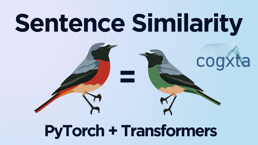
Gensim’s KeyedVectors comes into play for exploring sentence similarity. By making similarity queries, we unveil sentences closely related to a target sentence. This functionality provides a glimpse into the semantic connections within the dataset.
# Importing necessary libraries from gensim.models import KeyedVectors
# Saving embeddings to a file for Gensim
embedding_file = "sentence_embeddings.kv" with open(embedding_file, "w") as o:
o.write(f'{len(embeddings)} {len(embeddings[0])}\n') for text,
embedding in zip(texts[:len(embeddings)], embeddings):
text = re.sub("\s+", "_", text)
string_embedding = " ".join([str(v) for v in embedding])
o.write(f'{text} {string_embedding}\n')
# Loading embeddings with Gensim
sentence_vectors = KeyedVectors.load_word2vec_format('sentence_embeddings.kv', binary=False)
# Making similarity queries
sentence_vectors.most_similar(positive=["Hello."])
Clustering: Uncovering Patterns in Data
Explicitly clustering sentences adds another layer of exploration. We employ Scikit-learn’s AgglomerativeClustering to iteratively group similar sentences. The resulting clusters reveal patterns and common themes within the dataset.
# Importing necessary libraries
from sklearn.cluster import AgglomerativeClustering
import pandas as pd
# Clustering sentences
clusterer = AgglomerativeClustering(n_clusters=1000, affinity="euclidean", linkage="ward")
clusters = clusterer.fit_predict(embeddings)
# Creating a DataFrame for analysis
df = pd.DataFrame({"text": texts, "cluster": clusters})
# Analyzing specific clusters for cl in [200, 500, 800]:
print(df.loc[df['cluster'] == cl])
Conclusions: Unveiling the Power of Exploration
In this exploration journey, we’ve harnessed the capabilities of data visualization, sentence similarity, and clustering to understand the nuances within the Cornell Movie Dialogue Corpus. Beyond treating a dataset as a mere training ground, these techniques provide a holistic view. Robust NLP models require an understanding of the intricacies present in the data, allowing them to generalize effectively.
Whether you’re building chatbots, analyzing customer feedback, or diving into any NLP application, a thorough exploration of your textual data lays the foundation for success. Embrace the power of NLP in data exploration and unveil the stories hidden in your text.

